Getting Started
Import the energiscore library and other dependencies.
import energistream as es # Imports the Energiscore Library
import pandas as pd # Imports the Pandas Library for Dataframe handling
import datetime as dt # Imports the datetime Library for timeseries handling
import numpy as np # Imports the Numpy Library for series handling
import scipy as sp # Imports scipy package

import seaborn as sns # Imports seaborn for graph generation
import matplotlib # Imports matplotlib for math functionality
%load_ext autoreload
%autoreload 2
# Running autoreload will reload any updated modules before running a cell.
%pylab inline
%matplotlib inline
#pylab inline and matplotlib inline will cause charts to be displayed within ipython notebook.
Populating the interactive namespace from numpy and matplotlib
Client Instantiation and Authentication
EnergiStreamClient takes a valid username and password and establishes a unique session with temporary credentials.
Note : The following cell extracts the user credentials from an external text file to avoid displaying sensitive client information.
with open('../credentials.txt') as f:
    credentials = [x.strip().split(':') for x in f.readlines()]

USER = credentials[0][0]
PASS = credentials[0][1]
stream = es.EnergiStreamClient(USER, PASS, include_sensors=True)
External Data
get_weather returns a dataframe of hourly temperature and relative humidity data for the instantiated client’s associated physical location. Note : This data is collected from third party sources. Weather ID is an energistream unique key and not associated to any third party ID schema.
stream.get_weather(weather_id = 102, start = '12/29/2014', end = '1/29/2015').head()
| c | f | h | |
|---|---|---|---|
| 2014-12-29 00:00:00+00:00 | 15.6 | 60 | 42 |
| 2014-12-29 01:00:00+00:00 | 15.0 | 59 | 48 |
| 2014-12-29 02:00:00+00:00 | 13.3 | 56 | 55 |
| 2014-12-29 03:00:00+00:00 | 13.3 | 56 | 53 |
| 2014-12-29 04:00:00+00:00 | 12.2 | 54 | 57 |
Energistream Data and Metadata
get_energy accepts a sensor ID and returns a dataframe relating active and reactive energy, current and voltage RMS, and total Energy.
stream.get_energy(3505, start = '12/29/2014', end = '1/29/2015', tz = 'local').head()
| activeEnergy | currentRMS | powerFactor | reactiveEnergy | sensorId | totalEnergy | voltageRMS | |
|---|---|---|---|---|---|---|---|
| 2014-12-29 00:01:00-08:00 | 43566.626 | 27.44 | 0.93 | 13801.665 | 3505 | 45700.513 | 490.52 |
| 2014-12-29 00:02:00-08:00 | 43566.850 | 27.74 | 0.94 | 13801.740 | 3505 | 45700.749 | 490.00 |
| 2014-12-29 00:03:00-08:00 | 43567.077 | 30.02 | 0.93 | 13801.816 | 3505 | 45700.989 | 489.29 |
| 2014-12-29 00:04:00-08:00 | 43567.310 | 28.41 | 0.93 | 13801.901 | 3505 | 45701.236 | 491.54 |
| 2014-12-29 00:05:00-08:00 | 43567.541 | 27.81 | 0.94 | 13801.986 | 3505 | 45701.482 | 491.18 |
search_group_tree accepts a keyword and searches the instantiated client for matching sensor groups returning group names, sensor group ID, and assigned sensors.
stream.search_group_tree('Engineering',case=False).head()
| name | description | load_type | sensorGroups | sensors | groupMultiplier | time_zone | weatherStationId | base_group_level | |
|---|---|---|---|---|---|---|---|---|---|
| sensorGroupId | |||||||||
| 2177 | Rockwell Engineering Center - Sub Groups | Rockwell Engineering Center - Sub Groups | building | Int64Index([2179, 2178, 2180], dtype='int64') | None | [1, 1, 1] | America/Los_Angeles | 102 | 1 |
| 2258 | Engineering and Computing Trailer - Sub Groups | Engineering and Computing Trailer - Sub Groups | building | None | [{u'timeZoneId': 67, u'sourceTypeId': 1, u'des... | None | America/Los_Angeles | 102 | 1 |
| 157 | Engineering Laboratory Facility - Sub Groups | Feed to ELF Sub Loads | building | Int64Index([196, 193, 192, 195, 194], dtype='i... | None | [1, 1, 1, 1, 1] | America/Los_Angeles | 102 | 1 |
| 255 | Engineering Tower - Sub Groups | Feed to ET Sub Groups | building | Int64Index([258, 256, 257, 262, 263, 260, 261,... | None | [1, 1, 1, 1, 1, 1, 1, 1, 1] | America/Los_Angeles | 102 | 1 |
| 265 | Engineering Lecture Hall - Sub Groups | Feed ELH Sub Groups | building | Int64Index([274, 266, 271, 267, 270, 273, 272]... | None | [1, 1, 1, 3, 3, 3, 3] | America/Los_Angeles | 102 | 1 |
Sensors are grouped in a heirarchy by level.
stream.groups[stream.groups.base_group_level == 0].head()
| name | description | load_type | sensorGroups | sensors | groupMultiplier | time_zone | weatherStationId | base_group_level | |
|---|---|---|---|---|---|---|---|---|---|
| sensorGroupId | |||||||||
| 216 | UCI - MelRok Electric Meter Sub Groups | Feed to Individual Loads at UCI Buildings | campus | Int64Index([2203, 2193, 2198, 2188, 2177, 2181... | None | [1, 1, 1, 1, 1, 1, 1, 1, 1, 1, 1, 1, 1, 1, 1, ... | America/Los_Angeles | 102 | 0 |
| 734 | UCI - Electric Distribution Loads | Electrical Meters that Distribute Electricity ... | campus | Int64Index([732, 733, 1836, 1837, 1838, 1839, ... | None | [1, 1, 1, 1, 1, 1, -1, 1, 1] | America/Los_Angeles | 102 | 0 |
| 769 | UCI - Building Heating & Chilled Water Meters | 14 KEP-ES749 for 6 Buildings | campus | Int64Index([774, 775, 772, 771, 776, 777, 1824... | None | [1, 1, 1, 1, 1, 1, 1, 1, 1] | America/Los_Angeles | 102 | 0 |
| 1843 | UCI - Total Electric Load | Total Electric Load for UCI Campus | campus | Int64Index([735, 1842, 1484, 1483, 1486, 1485,... | None | [1, 1, 1, 1, 1, 1, 1, 1, 1, 1, 1, 1, 1, 1, 1, ... | America/Los_Angeles | 102 | 0 |
sensors returns a dataframe describing the individual sensors associated with the instantiated energistream client ID. This includes the sensor ID, the associated group ID, time zone, and a multiplier based on the method of measurement i.e. one, two, or three channel.
stream.sensors.head()
| description | iconId | multiplier | name | properties | sensorFunctionTypeId | sensorGroupId | sourceTypeId | time_zone | |
|---|---|---|---|---|---|---|---|---|---|
| sensorId | |||||||||
| 8812 | D40010000628-04 | 21 | 1 | ECT B1 | [{u'name': u'Phase', u'value': u'A'}] | 1 | 2258 | 1 | America/Los_Angeles |
| 8813 | D40010000628-05 | 21 | 1 | ECT B2 | [{u'name': u'Phase', u'value': u'C'}] | 1 | 2258 | 1 | America/Los_Angeles |
| 8814 | D40010000628-06 | 21 | 1 | ECT B3 | [{u'name': u'Phase', u'value': u'B'}] | 1 | 2258 | 1 | America/Los_Angeles |
| 8815 | D40010000628-07 | 21 | 1 | ECT B4 | [{u'name': u'Phase', u'value': u'A'}] | 1 | 2258 | 1 | America/Los_Angeles |
| 8816 | D40010000628-08 | 21 | 1 | ECT B5 | [{u'name': u'Phase', u'value': u'C'}] | 1 | 2258 | 1 | America/Los_Angeles |
get_boards returns a dataframe describing the boards associated with the instantiated energistream client ID. This includes the boards serial number, version, display name, and model.
stream.get_boards.head()
| currentConfigVersion | displayName | firmwareVersion | manufacturer | model | sensors | timeZoneId | |
|---|---|---|---|---|---|---|---|
| serialNumber | |||||||
| C20006000002 | 26 | MSTB First Floor 2 | 1 | MelRok Manufacturer | EN-12 | [{u'timeZoneId': 67, u'sourceTypeId': 1, u'nam... | 67 |
| C20006000003 | 21 | MSTB First Floor 3 | 1 | MelRok Manufacturer | EN-12 | [{u'timeZoneId': 67, u'sourceTypeId': 1, u'nam... | 67 |
| C20006000004 | 25 | MSTB Second Floor | 1 | MelRok Manufacturer | EN-12 | [{u'timeZoneId': 67, u'sourceTypeId': 1, u'nam... | 67 |
| A30006000036 | 20 | Aldrich Hall | 1 | MelRok Manufacturer | EN-12 | [{u'timeZoneId': 67, u'sourceTypeId': 1, u'nam... | 67 |
| A30006000041 | 18 | Social Science LAB | 1 | MelRok Manufacturer | EN-12 | [{u'timeZoneId': 67, u'sourceTypeId': 1, u'nam... | 67 |
get_demand returns the fifteen minute demand rate for the given sensor group. Start and end date may be specified as well as the timezone and desired resolution. Note : Defaults to the last thirty days and fifteen minute resolution.
stream.get_demand(157).head()
2015-02-05 13:44:59-08:00     43.339200
2015-02-05 13:59:59-08:00     44.102333
2015-02-05 14:14:59-08:00     79.040466
2015-02-05 14:29:59-08:00    131.523733
2015-02-05 14:44:59-08:00     45.773866
Name: kW, dtype: float64
Presentation and Analysis Examples
seaborn is used to plot aesthetically pleasing charts and graphs. The following commands set up the presentation by defining the seaborn aesthetics, chart sizing, and figure scaling to be used. .. code:: python
sns.set(font=’Bitstream Vera Sans’) sns.set_context(‘poster’) #sns.set_context(“poster”, font_scale=1.7) sns.plotting_context()
{'axes.labelsize': 17.6,
 'axes.titlesize': 19.200000000000003,
 'figure.figsize': array([ 12.8,   8.8]),
 'grid.linewidth': 1.6,
 'legend.fontsize': 16.0,
 'lines.linewidth': 2.8000000000000003,
 'lines.markeredgewidth': 0.0,
 'lines.markersize': 11.200000000000001,
 'patch.linewidth': 0.48,
 'xtick.labelsize': 16.0,
 'xtick.major.pad': 11.200000000000001,
 'xtick.major.width': 1.6,
 'xtick.minor.width': 0.8,
 'ytick.labelsize': 16.0,
 'ytick.major.pad': 11.200000000000001,
 'ytick.major.width': 1.6,
 'ytick.minor.width': 0.8}
A large dataset at a sufficiently fine resolution may contain very large short duration demand spikes which are not indicative of the actual demand. These spikes may be filtered out, carefully, by masking demand values that exceed a defined limit. .. code:: python
demand = stream.get_demand(216) multi = 1.5 mask = (demand < 0) | (demand > demand.mean() + multi * demand.std())
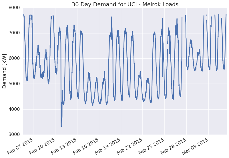
Seen below is the demand charted over a thirty day time period. This can provide insight into demand over time such as due to changes in the weather or building usage. Note the regularly spaced peaks during the work-day and comparatively smaller spikes which occur on off-days. There is a three day period of reduced demand coinciding with February 16th, a Federal Holiday. .. code:: python
demand.mask(mask).plot()
plt.title(‘30 Day Demand for UCI - Melrok Loads’) plt.ylabel(‘Demand [kW]’)
<matplotlib.text.Text at 0x11659c790>
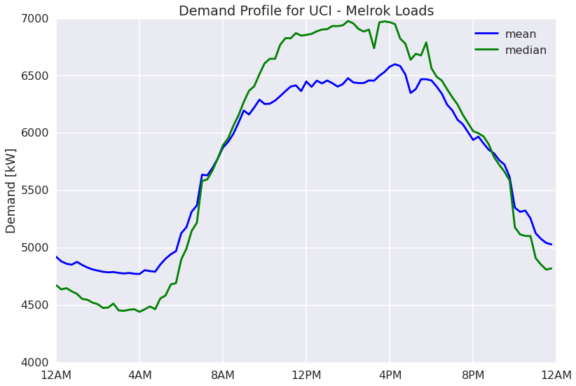
Taking the mean and median of the days creates a single chart representing an average demand day. This is useful for examining a typical demand profile such as to obverve the time of peak loads and the duration of regular demand spikes. In this case the peak occurs in the middle of the afternoon around 3 PM. Comparing the mean and median offers quick insight into the daily variation in demand. .. code:: python
mean = demand.mask(mask).groupby([demand.index.hour,demand.index.minute]).mean().plot(color = ‘b’, label = ‘mean’) median = demand.mask(mask).groupby([demand.index.hour,demand.index.minute]).median().plot(color = ‘g’, label = ‘median’) legend()
plt.title(‘Demand Profile for UCI - Melrok Loads’) plt.ylabel(‘Demand [kW]’)
plt.xticks( (16 * arange(7)),[‘12AM’,‘4AM’,‘8AM’,‘12PM’,‘4PM’,‘8PM’,‘12AM’])
([<matplotlib.axis.XTick at 0x11659c050>,
  <matplotlib.axis.XTick at 0x112f7b810>,
  <matplotlib.axis.XTick at 0x1168cf290>,
  <matplotlib.axis.XTick at 0x1168cfa50>,
  <matplotlib.axis.XTick at 0x1168c7210>,
  <matplotlib.axis.XTick at 0x1168c7990>,
  <matplotlib.axis.XTick at 0x1168b9090>],
 <a list of 7 Text xticklabel objects>)
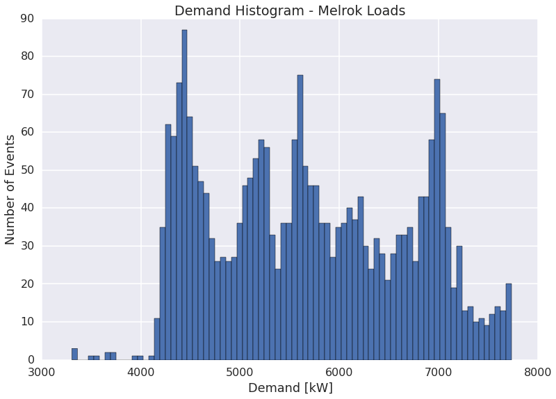
A histogram is another useful way to examine the distribution of the demand, plotting demand magnitude by the total number of events in the data set. .. code:: python
demand.mask(mask).hist(bins=80)
plt.title(‘Demand Histogram - Melrok Loads’) plt.ylabel(‘Number of Events’) plt.xlabel(‘Demand [kW]’)
<matplotlib.text.Text at 0x1168ee210>